EEG experiments record the electrical activity of the brain while participants rest, perform tasks or receive stimuli. EEG has millisecond temporal resolution but limited spatial resolution (see Introduction to EEG). This tutorial covers the planning and design of EEG experiments: paradigms, approaches to analysis, triggers and the number of trials.
Equipment
Electrodes: from a few to 256, usually mounted in a cap at standard positions (10-20 or 10-10 system), plus EOG, ECG and EMG electrodes when needed.
Amplifier: amplifies the microvolt signals and digitizes them (analog-to-digital converter, usually 24 bits).
Recording computer: stores the data together with the event markers (triggers).
Stimulus computer: presents the stimuli and sends triggers to the amplifier.
Steps of an EEG experiment
Research question and hypotheses: which brain activity or cognitive process is studied (e.g. attention, memory, sleep, epilepsy)?
Paradigm: the task or stimulation (e.g. resting state, oddball paradigm for the P300, steady-state stimulation).
electrode placement (10-20 system or high-density arrays) and impedance check (e.g. < 5–10 kΩ for passive electrodes)
resting-state recordings (e.g. eyes open and closed) as a reference
the task, with triggers marking the events
Preprocessing: filtering (e.g. 0.1–40 Hz for ERPs, 0.5–45 Hz for spectral analysis), artifact removal (e.g. ICA for blinks), re-referencing (e.g. average reference).
Analysis: time domain (ERPs, e.g. P300, N170), frequency domain (band powers), time-frequency domain (wavelets, short-time Fourier transform), connectivity.
Statistics and interpretation: linking EEG features to cognitive or clinical variables (e.g. t-tests, ANOVA, mixed models, permutation tests, machine learning).
Common paradigms
Event-related potentials (ERPs): averaged responses time-locked to stimuli or responses (e.g. P300 in the oddball paradigm), see ERPs/ERFs.
Resting-state EEG: spontaneous activity with eyes open or closed (e.g. alpha rhythm).
Steady-state evoked potentials (SSEPs): responses to periodic (e.g. flickering) stimuli at the stimulation frequency.
Event-related (de)synchronization: changes of oscillatory power during tasks (e.g. motor imagery).
Artifacts: eye movements and blinks, muscle activity, movements, sweating, line noise.
Spatial resolution: volume conduction smears the potentials over the scalp, and deep sources contribute little.
Interpretation: scalp signals are mixtures of many sources; the reverse inference from EEG features to cognitive processes needs caution.
Applications: clinical diagnostics (epilepsy, sleep disorders, coma, brain injury), cognitive neuroscience (perception, attention, memory, language), psychiatry and pharmacology, brain-computer interfaces (spellers, control of devices).
Planning an Experiment
Example: hypothesis: alpha power (8–12 Hz) over occipital channels is higher with eyes closed than with eyes open; experiment: resting-state EEG with alternating periods of eyes open and closed; analysis: band power compared between conditions (e.g. paired t-test).
Literature review: what is known, which methods were used, what were their limitations; adapt your design accordingly.
movement artifacts: comfortable seating, a chin rest, instructions to relax and avoid movements
muscle artifacts: avoid tasks with speech, chewing or strong facial and neck muscle activity during the periods of interest
eye artifacts: a fixation cross, blink breaks between trials
line noise: keep electrical devices away, use a shielded room if available
Number of trials: enough to obtain a reliable signal (see Estimating the number of trials); the required number depends on the size of the effect: large components (e.g. P300) need fewer trials than small ones (e.g. early sensory components, small differences between conditions), and trials are lost to artifact rejection. Balance the number of trials with the fatigue of the participant.
Simple design: test one hypothesis with a minimal number of conditions; complex multi-task paradigms make interpretation difficult.
Power analysis: estimate the sample size needed to detect the expected effect (from previous studies or pilot data) with the chosen significance level and power (typically 0.8), e.g. with G*Power or simulations.
Pre-registration: register the hypotheses, methods and analysis plan before data collection (e.g. OSF, AsPredicted; ClinicalTrials.gov for clinical trials); it separates confirmatory from exploratory analyses and reduces flexibility in data analysis (“p-hacking”).
Stimulus timing: check the actual timing of stimuli and triggers with a photodiode (visual) or a microphone (auditory); a 60 Hz monitor shows a new frame every 16.7 ms, so visual onsets are quantized and may be delayed.
Pilot testing: run the whole procedure (setup, task, recording, analysis) on 1–3 pilot participants and adjust the protocol.
Environment: a comfortable temperature (about 20–22 °C; sweating causes slow drifts of the signal), dim but sufficient light, a quiet room.
Documentation: participant ID, date, time, impedances, and all unusual events (e.g. “participant moved at 10:23”, “electrode Fz lost contact; re-applied gel”).
Data organization: use the Brain Imaging Data Structure (BIDS) for file naming (e.g. sub-01_task-nback_eeg.set) and metadata (channels, electrode positions, events).
No changes during data collection: do not modify the paradigm, equipment or analysis plan once the data collection has started; if unavoidable, document the change and evaluate its effect.
After the study, review what worked and what did not, to improve future experiments.
Approaches to Analysis
Exploratory and Hypothesis-Driven Analyses
Hypothesis-driven (confirmatory) analyses test specific predictions defined before the data are seen (ideally pre-registered): e.g. “the P300 amplitude at Pz in the 300–500 ms window is larger for targets than for standards”. The number of tests is small, so the statistical power is high and few corrections for multiple comparisons are needed.
Exploratory analyses search the data for patterns without strong a priori predictions, e.g. testing all channels, time points and frequencies. They can reveal unexpected effects and generate hypotheses, but the large number of tests requires a correction for multiple comparisons (e.g. FDR, cluster-based permutation tests), which reduces the sensitivity, and their results should be confirmed in independent data.
novel questions, pilot studies, secondary analyses
confirmation, replication, theory testing
Both are legitimate if they are reported as what they are. A common combination: exploratory analyses in one dataset (or one part of the data), followed by confirmatory tests in independent data.
Choice of statistical tests: parametric tests (t-tests, ANOVA, regression, mixed models) assume e.g. normally distributed residuals; non-parametric and permutation tests make fewer assumptions and handle the dependencies between neighbouring channels, times and frequencies (cluster-based permutation tests). Both can be used in exploratory and confirmatory analyses.
Subject-Level and Group-Level Analyses
Subject-level (single-subject) analyses test effects within one participant, across trials: e.g. whether a patient shows an ERP component, or whether a BCI user’s motor imagery can be classified. They describe individuals (clinical diagnostics, BCIs, case studies) but do not generalize to a population, and they require effects that are large relative to the trial-to-trial variability.
Group-level analyses test whether an effect is consistent across participants (e.g. the mean of the participants’ averages), generalizing to the population from which the sample was drawn. They are the basis of most experimental and clinical studies (e.g. patients vs. controls), but may hide individual differences (an effect present in some participants and absent in others).
Feature
Subject-level
Group-level
Unit of analysis
trials of one participant
participants
Generalization
to this participant
to the population
Variability
trial-to-trial
between participants
Effects detected
large, within-subject effects
small but consistent effects
Use
case studies, clinical diagnostics, BCIs
experiments, clinical comparisons
Both levels are combined in mixed-effects (hierarchical) models, which model the variability between trials and between participants at the same time, and in the common two-step approach: averages (or statistics) per participant, then a group test.
Event-Related Experiments
In event-related designs, brain activity is time-locked to discrete events (stimuli or responses) repeated many times, and the responses are averaged (ERPs) or analyzed in the time-frequency domain.
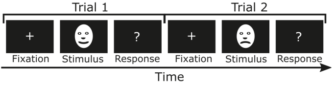
A typical trial:
Fixation (e.g. 500–1000 ms): a fixation cross; the pre-stimulus interval serves as the baseline.
Stimulus (e.g. 200–2000 ms, depending on the stimulus), e.g. faces with happy or angry expressions as two conditions.
Response: a button press or another response; responses generate their own brain activity.
Inter-trial interval: usually jittered (randomly varied, e.g. 1000–1500 ms), so that the participant cannot anticipate the next stimulus and the anticipatory activity and the alpha rhythm are not time-locked to the stimulus.
Considerations:
Variable timing: processes whose latency varies between trials (e.g. decisions) are smeared by averaging; time-frequency or single-trial analyses, or response-locked averages, capture them better.
Motor responses: button presses generate their own potentials (the readiness potential before, motor potentials after the movement), which overlap with late stimulus-related components; delay the response (e.g. after a cue), use conditions without responses, or analyze response-locked averages.
Overlap: with short intervals between stimuli, the responses to consecutive stimuli overlap; a jittered interval reduces the overlap with the baseline, and regression-based methods (deconvolution) can separate overlapping responses.
Baseline: the pre-stimulus interval must be free of activity related to the previous trial or to anticipation.
Artifacts: blinks and eye movements are frequent after the stimulus; instruct participants to blink between trials and to keep fixation.
Randomization and counterbalancing: randomize the order of the conditions and counterbalance stimuli and response hands across participants, so that differences between conditions are not caused by order, fatigue or stimulus features.
Block Designs and Steady-State Responses
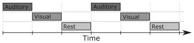
In block (boxcar) designs, each condition is presented continuously for a longer period (e.g. 10–60 s), alternating with other conditions or rest; the sustained (tonic) activity, e.g. oscillatory power, is compared between blocks. Event markers mark the onset of each block.
Long blocks are sensitive to slow changes (fatigue, drowsiness, electrode drift) and to the order of the conditions; counterbalance or randomize the order of blocks.
Steady-state evoked potentials (SSEPs): a stimulus modulated at a fixed frequency (e.g. a visual stimulus flickering at 12 Hz) evokes a response at that frequency and its harmonics, measurable as a narrow peak in the spectrum with a high signal-to-noise ratio.
Frequency tagging: two stimuli presented at the same time, modulated at different frequencies (e.g. 12 and 15 Hz), can be separated in the frequency domain, e.g. to measure the attention paid to each of them. Simulated occipital EEG (pink noise) with 12 and 15 Hz steady-state responses of 1 μV:
Although the steady-state responses are 10 times smaller than the background EEG (standard deviation 10 μV), they are visible as narrow peaks at 12 and 15 Hz, because the background power is spread over all frequencies while the responses are concentrated at the stimulation frequencies. A long recording (and a fine frequency resolution) increases the signal-to-noise ratio of the peaks.
Triggers
Triggers (event markers) mark the times of events (stimuli, responses, block onsets) in the EEG recording, so that the data can be segmented into epochs and averaged.
Transmission:
Parallel port / TTL triggers: the stimulus computer sets a number of digital lines (usually 8, using TTL logic levels) for a short time (e.g. 5–50 ms); the value of the lines (0–255) is recorded as the trigger code.
USB or network triggers (e.g. Lab Streaming Layer, LSL): events are sent as timestamped messages; precise synchronization of the clocks of the stimulus and recording computers is essential.
Analog signals: e.g. a photodiode on the screen or a microphone recorded on an auxiliary channel, measuring the actual stimulus onset.
Responses: response boxes send their own triggers.
Source
Example
Trigger
Stimulus presentation
onset of a visual or auditory stimulus
TTL code (e.g. 1 = condition A)
Behavioural responses
button press
TTL code from a response box
Physiological events
R peaks of the ECG, blinks
detected later from the recorded signals
External devices
MRI scanner volumes, eye tracker
TTL pulses or synchronization messages
Problems:
Delays: a constant delay between the trigger and the actual stimulus (e.g. the time the monitor needs to draw the image, audio buffering); measure it (photodiode, microphone) and correct the event times.
Jitter: a variable delay (e.g. a stimulus waiting for the next monitor refresh, non-real-time operating systems); it smears the averaged responses and cannot be corrected by a constant shift; use a photodiode or software with precise timing (e.g. Psychtoolbox, PsychoPy).
Missed or extra triggers: check the number of triggers of each type against the experiment log.
Best practices:
Test the whole chain (stimulus, trigger, recording) in pilot sessions and inspect the triggers in the recorded data.
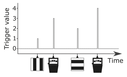
Keep a trigger code legend, e.g.:
Trigger
Event
1
happy face
2
angry face
3
correct response
4
incorrect response
Log the events in the stimulus software as well, to cross-check the triggers.
Correct measured constant delays before epoching.
Example: a happy face appears on the screen; the stimulus computer sends trigger 1 at the moment the image is displayed; in the analysis, epochs from −200 to 800 ms around trigger 1 are averaged to obtain the ERP to happy faces. In NeuroAnalyzer, triggers are stored in obj.markers and used by epoch(obj; marker = ...).
The figure shows triggers as short pulses marking the times of events in the recording.
Estimating the Number of Trials
How many trials are needed for a reliable estimate depends on the size of the effect relative to the trial-to-trial variability (the signal-to-noise ratio of single trials). It can be estimated from pilot data with the split-half reliability: two independent random sets of \(n\) trials each are averaged, the two averages are correlated, and the correlation is plotted against \(n\). The correlation increases with \(n\) and approaches a plateau: adding further trials improves the reliability only a little. Unlike correlating partial averages with the average of all trials (which contains the same trials and reaches 1 by construction), the two halves are independent.
Simulated ERP (a P300-like wave of 8 μV, or a smaller component of 3 μV) with single-trial noise of 10 μV (pink noise), 200 baseline-corrected trials:
fs =250t =collect(-0.2:(1/ fs):0.8)n_t =length(t)n_trials =200# pink noise with standard deviation 10 μVfunctionnoise() x =generate_noise(n_t; type=:pink)return10.* (x .-mean(x)) ./std(x)enderp(a) = a .*exp.(-(t .-0.35) .^2./ (2*0.06^2))bl = t .<0# time × trials, baseline-correctedfunctiontrials(a) x =hcat([erp(a) .+noise() for _ in1:n_trials]...)return x .-mean(x[bl, :]; dims =1)endx_large =trials(8)x_small =trials(3)# split-half reliability for n trials per half (100 random splits)functionsplit_half(x, n) r =zeros(100)for k in1:100 idx = NeuroAnalyzer.Random.randperm(size(x, 2)) avg1 =vec(mean(x[:, idx[1:n]]; dims =2)) avg2 =vec(mean(x[:, idx[(n +1):(2n)]]; dims =2)) r[k] =cor(avg1, avg2)endreturnmedian(r)end
ns =2:2:100fig, ax =lines(ns, [split_half(x_large, n) for n in ns]; label ="8 μV component", figure = (size = fig_size,), axis = (ax_style..., xlabel ="Number of trials (per half)", ylabel ="Split-half correlation"))lines!(ax, ns, [split_half(x_small, n) for n in ns]; color =:red, label ="3 μV component")hlines!(ax, 0.8; color =:black, linestyle =:dash)axislegend(ax; position =:rb)fig
The 8 μV component reaches a split-half correlation of 0.8 with about 50–60 trials per half, while the 3 μV component remains unreliable even with 100 trials per half: the number of trials needed increases with the square of the noise-to-signal ratio (a component 2.7 times smaller needs about 7 times more trials). In real data, the same analysis on pilot recordings (e.g. for the waveform, the mean amplitude in a time window, or the power in a frequency band) indicates the number of trials needed, to which the expected loss of trials to artifact rejection must be added.
The correlation of the waveforms is calculated over the whole epoch, including the baseline where there is only noise; for a specific measure (e.g. the mean amplitude in a time window), the reliability of that measure across subsets of trials can be calculated instead. For skewed, non-negative measures such as power, the Spearman (rank) correlation is more robust than the Pearson correlation used here.