Electroencephalography (EEG) records the electrical activity of the brain with electrodes placed on the scalp. This tutorial explains where the EEG signal comes from, how it travels to the scalp and how it is recorded.
The Brain in Numbers
Quantity
Approximate value
Neurons in the human brain
\(8.6 \times 10^{10}\) (about 16 billion in the cerebral cortex)
Synapses
\(10^{14}\)–\(10^{15}\)
Neuron density in the neocortex
\(2\)–\(10 \times 10^4\) per mm³
Neurons under 1 mm² of cortical surface
about \(10^5\), 70–80% of them pyramidal neurons
Thickness of the neocortex
2–4 mm (six layers)
Synaptic delay
0.5–1 ms
Scalp EEG amplitude
10–100 μV
The neocortex is the outer layer of the cerebral hemispheres, responsible for perception, cognition and voluntary movement. It has six layers with distinct types of neurons and connections. Pyramidal neurons are its principal (excitatory) neurons; their long apical dendrites are aligned in parallel, perpendicular to the cortical surface, which makes them the main generators of the EEG.
expensive, shielded room, insensitive to radial sources
fMRI
blood oxygenation (BOLD)
seconds
millimeters
whole brain, deep structures
slow, indirect (hemodynamic) measure
fNIRS
hemoglobin concentration (near-infrared light)
seconds (hemodynamic)
1–3 cm
portable, tolerant to movement
only superficial cortex, indirect measure
EEG was first recorded in humans by Hans Berger in 1924 (published in 1929). It is used in clinical neurophysiology (epilepsy, sleep, disorders of consciousness, anesthesia monitoring) and in research on perception, cognition and brain states (e.g. resting state with eyes closed and open, task-related activity, event-related potentials).
Invasive and non-invasive recordings of electrical activity differ in scale:
Recording
Electrodes
Signal
Spatial scale
Intracellular recording
inside a neuron (sharp electrode, patch clamp)
membrane potential of one neuron
single cell
Single unit / multi-unit recording
extracellular microelectrodes in brain tissue
action potentials (spikes) of one or a few neurons
field potentials of deep and superficial structures
millimeters
Scalp EEG
electrodes on the scalp
summed activity of large cortical areas
centimeters
ECoG and sEEG are collectively called intracranial EEG (iEEG); they are recorded in patients (e.g. before epilepsy surgery), see Intracranial EEG below. Single unit and LFP recordings use the same intracortical electrodes (high-pass and low-pass filtered signals, respectively); in humans they are possible only during neurosurgical procedures.
Resting Potential
The resting potential (\(V_m\)) is the potential difference across the membrane of a neuron at rest: typically −60 to −80 mV (inside negative). It is maintained by concentration gradients of ions (kept by ATP-dependent pumps, e.g. the Na⁺/K⁺ pump) and by the selective permeability of the membrane.
The equilibrium (Nernst) potential of an ion is the membrane potential at which the electrical force exactly balances the concentration gradient, so that there is no net flow of the ion:
where \(R\) is the gas constant, \(T\) the absolute temperature, \(z\) the charge of the ion and \(F\) the Faraday constant (\(RT/F \approx 26.7\) mV at 37 °C).
At rest, the membrane is mostly permeable to K⁺ (through leak channels). K⁺ flows out of the cell down its concentration gradient, leaving the inside negative, until the electrical force pulling K⁺ back balances the gradient (−80 mV). A small permeability to Na⁺ shifts the resting potential towards the Na⁺ equilibrium potential, so the actual resting potential (about −70 mV) lies between the equilibrium potentials of K⁺ and Na⁺, weighted by the permeabilities (the Goldman equation).
Although small, the membrane potential is large relative to the thickness of the membrane (about 5 nm): the electric field across the membrane is about \(0.07 / 5 \times 10^{-9} \approx 10^7\) V/m.
Action Potential
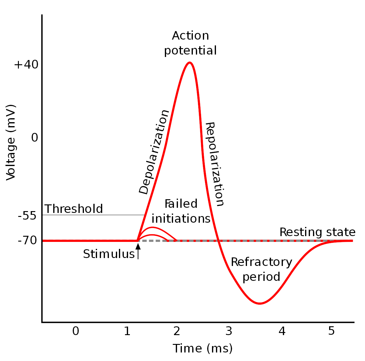
An action potential is a rapid, transient reversal of the membrane potential, propagating along the axon, by which neurons transmit information over long distances.
Amplitude: about 100 mV (from −70 mV to about +30 mV).
Duration: about 1 ms (1–2 ms including repolarization).
Phases:
Depolarization: a stimulus depolarizes the membrane to the threshold (about −55 mV); voltage-gated Na⁺ channels open and Na⁺ influx depolarizes the membrane further, to a positive overshoot.
Repolarization: Na⁺ channels inactivate and voltage-gated K⁺ channels open; K⁺ efflux returns the membrane potential towards rest.
Afterhyperpolarization: K⁺ channels close slowly, so the membrane potential transiently falls below the resting potential (for several milliseconds).
Refractory periods: during the absolute refractory period (depolarization and most of the repolarization, while Na⁺ channels are inactivated) no new action potential can be generated; during the relative refractory period (afterhyperpolarization) a stronger stimulus is needed.
The Na⁺/K⁺ pump restores the ion gradients over a longer time scale.
Propagation: the action potential spreads along the axon by local currents that depolarize the neighbouring membrane. The distance over which a potential change decays to 37% along a passive fiber is the space constant:
\[
\lambda = \sqrt{\frac{d R_m}{4 R_i}}
\]
where \(d\) is the axon diameter, \(R_m\) the specific membrane resistance and \(R_i\) the resistivity of the axoplasm. Thicker axons (and myelination, which increases \(R_m\)) propagate potentials further and faster. Rapidly changing potentials decay faster than \(\lambda\) predicts, because part of the current charges the membrane capacitance.
Sources of the EEG
The EEG is generated mainly by postsynaptic potentials (PSPs) of cortical pyramidal neurons, not by action potentials:
An excitatory postsynaptic potential (EPSP) is a depolarization caused by an inflow of positive ions (mainly Na⁺) at an excitatory synapse.
An inhibitory postsynaptic potential (IPSP) is a hyperpolarization caused by an inflow of Cl⁻ or an outflow of K⁺ at an inhibitory synapse.
PSPs last 10–100 ms and have amplitudes of up to a few millivolts (much less than an action potential).
PSPs spread along the dendrites to the soma and are summed (spatially and temporally) at the axon hillock; if the membrane potential reaches the threshold (about −50 to −55 mV), an action potential is generated. At the axon terminal, the action potential opens voltage-gated Ca²⁺ channels; the Ca²⁺ influx triggers the release of neurotransmitter, which generates PSPs in the next neuron. An inhibitory synapse close to an excitatory one can also shunt the excitatory current (shunting inhibition), reducing the depolarization without causing a hyperpolarization.
Why PSPs and not action potentials? Action potentials are short (about 1 ms) and biphasic; even small timing differences between neurons make them cancel out. PSPs are slow and monophasic, so the PSPs of many neurons overlap in time and sum up.
Dipoles
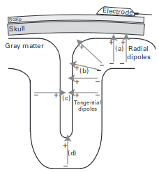
An EPSP at the apical dendrite of a pyramidal neuron causes an inflow of positive charge into the cell: the extracellular space at the synapse becomes negative (a current sink). The current flows along the dendrite inside the cell and leaves the cell at other sites (a current source, extracellularly positive), closing the loop in the extracellular space. The pair of sink and source forms a current dipole aligned with the somatodendritic axis.
For a source in a homogeneous conductor of conductivity \(\sigma\), the potential at the distance \(r\):
monopole (a single source or sink of current \(I\)): \(V = \dfrac{I}{4 \pi \sigma r}\), falling off with \(1/r\)
dipole (a source and a sink \(d\) apart, \(r \gg d\)): \(V = \dfrac{I d \cos\theta}{4 \pi \sigma r^2}\), falling off with \(1/r^2\); \(\theta\) is the angle between the dipole axis and the direction to the measurement point
quadrupole (two opposite dipoles, e.g. an action potential travelling along an axon): falling off with \(1/r^3\)
r =linspace(1, 10, 100)fig, ax =lines(r, 1./ r; label ="monopole (1/r)", figure = (size = fig_size,), axis = (ax_style..., xlabel ="Distance [AU]", ylabel ="Relative potential", yscale = log10))lines!(ax, r, 1./ r .^2; color =:red, label ="dipole (1/r²)")lines!(ax, r, 1./ r .^3; color =:green, label ="quadrupole (1/r³)")axislegend(ax; position =:rt)fig
The fields of action potentials (quadrupoles) fall off fast and cancel out; the dipolar fields of synchronously activated PSPs reach the scalp.
Polarity at the scalp depends on the location of the synapses: an EPSP at superficial synapses (close to the cortical surface) creates a sink near the surface and gives a negative potential at the scalp; an EPSP at deep synapses creates a superficial source and gives a positive potential. IPSPs have the opposite polarity. The scalp polarity alone therefore does not tell whether the underlying activity is excitatory or inhibitory.
Synchronization and Orientation
A scalp electrode records the sum of the fields of many neurons. A measurable signal requires:
synchrony: tens of thousands of neurons must be activated at the same time (a MEG-detectable dipole of 10 nAm corresponds to about 50 000 simultaneously active pyramidal neurons); the spontaneous scalp EEG reflects synchronized activity of 6–10 cm² of cortex
parallel orientation: the dipoles must point in the same direction; the aligned pyramidal neurons of layers III and V are the main generators, while neurons with radially symmetric dendrites (closed fields) produce no external field
The orientation of the dipoles relative to the sensors matters:
Radial dipoles (perpendicular to the scalp, e.g. at the crown of a gyrus) are best detected by EEG and invisible to MEG.
Tangential dipoles (parallel to the scalp, e.g. in the walls of a sulcus) are well detected by MEG and less well by EEG.
Dipoles of opposite orientation (e.g. on the two walls of a sulcus) cancel each other.
Other contributions: glial cells contribute to slow and infraslow potentials (< 0.1 Hz); highly synchronized action potentials (bursts) can contribute to high-frequency activity in the LFP.
Volume Conduction
The tissues of the head (brain, cerebrospinal fluid, skull, scalp) form a volume conductor: the currents generated in the cortex flow through the whole head, and the scalp potential at every electrode is a weighted sum of the activity of all sources.
Linearity: volume conduction is linear (superposition): the scalp potentials of several sources add up.
Instantaneous: at EEG frequencies the capacitive properties of the tissues can be neglected; the potentials appear at all electrodes at the same time (zero phase lag), which is important for connectivity analysis.
Smearing: the skull has a low conductivity (about 1/15–1/80 of that of the brain and scalp), which spreads the potential of a small cortical source over a large area of the scalp. A single EEG channel reflects activity from about 10 cm² of cortex.
Depth: the amplitude decreases with distance (with \(1/r^2\) for dipoles), so the EEG is dominated by superficial cortical sources; deep structures (thalamus, hippocampus, brainstem) contribute little.
Head models used to calculate scalp potentials range from a homogeneous sphere, through concentric spheres with different conductivities (brain, CSF, skull, scalp), to realistic models built from the individual MRI (boundary or finite element methods).
Forward and inverse problems:
The forward problem: calculating the scalp potentials of known sources; it has a unique solution for a given head model.
The inverse problem: estimating the sources (location, orientation, strength) from the scalp potentials; it has no unique solution (infinitely many source configurations produce the same scalp potentials) and must be constrained by assumptions (e.g. a small number of dipoles, sources in the cortex, minimum norm) and anatomical information (MRI).
High-density EEG (64–256 electrodes) samples the scalp potential better and improves source localization; spatial filters (e.g. the surface Laplacian or current source density) reduce the effect of volume conduction.
Recording the EEG
Differential Amplification
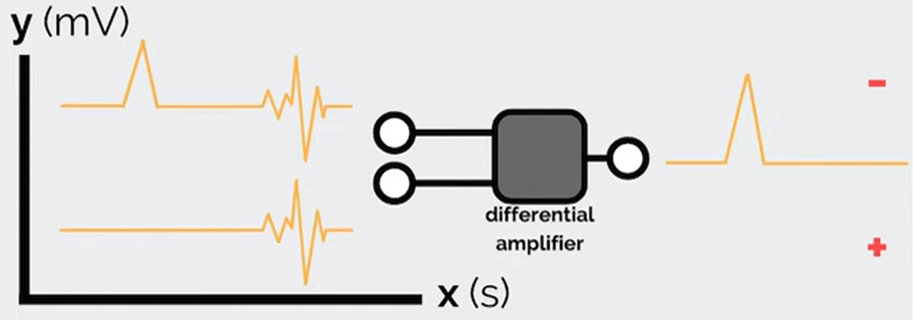
An EEG amplifier measures the difference between the potentials of two inputs, so every EEG channel is a potential difference between two electrodes:
\[
V_{out} = (V_1 - V_2) \times \text{gain}
\]
Interference common to both inputs (e.g. power-line noise picked up by the body) is suppressed. The ability to suppress it is the common mode rejection ratio (CMRR), the ratio of the gain for the difference signal to the gain for the common signal, usually given in dB (EEG amplifiers: > 100 dB):
The ground electrode connects the subject to the amplifier ground, which is necessary for common mode rejection; its position does not affect the recorded signals if its impedance is low. The reference is the second input: in a referential montage all channels share one reference electrode (e.g. Cz, the mastoids or the earlobes, or a reference computed later, e.g. the average reference); in a bipolar montage each channel is the difference of two neighbouring electrodes. See Montages and Referencing.
Polarity Convention
In clinical EEG, negative potentials are displayed upwards (input 1 more negative than input 2 gives an upward deflection).
Example (bipolar chain F8–T8–P8 with a negative potential maximal at T8):
The deflections in the two channels point in opposite directions: this phase reversal marks the electrode shared by the two channels (T8) as the location of the maximum (or minimum) of the potential. Phase reversals in bipolar montages are used to localize focal activity, e.g. epileptic spikes.
Because every channel is a difference, the EEG is always relative: the amplitude and shape of a channel depend on the reference.
Gain, Resolution and Noise
The EEG is small (microvolts), so it must be amplified before it is digitized. Gains are expressed in dB: \(\text{dB} = 20 \log_{10}(V_{out} / V_{in})\). Older amplifiers used gains of thousands to a million; modern DC-coupled amplifiers with 24-bit analog-to-digital converters need much lower gains, because their resolution is fine enough (a fraction of a microvolt) to record the EEG directly.
Typical magnitudes:
scalp EEG: 10–100 μV (up to 200 μV in children and in deep sleep); event-related potentials: 1–10 μV
amplifier noise: < 1 μV (RMS)
power-line interference picked up by the body: up to millivolts (removed by common mode rejection and, if necessary, by filtering)
Electrodes and Impedance
The amplifier draws a small current from the source; the measured voltage \(V'\) depends on the ratio of the input impedance of the amplifier (\(R_i\)) and the impedance of the source and electrode (\(R_o\)):
\[
V' = V \frac{R_i}{R_i + R_o}
\]
The input impedance of the amplifier must therefore be much higher than the electrode impedance (EEG amplifiers: > 100 MΩ).
The electrode-skin impedance should be low and similar across electrodes (unequal impedances reduce common mode rejection): traditionally < 5 kΩ for passive electrodes (< 10–20 kΩ for modern high-impedance amplifiers; active electrodes tolerate higher values). It is reduced by cleaning and gently abrading the skin and by conductive gel or paste.
Types of electrodes:
Material: silver/silver chloride (Ag/AgCl) electrodes are standard: they are non-polarizable and record slow potentials without drift; gold, tin and stainless steel are also used.
Wet electrodes: conductive gel, paste or saline (sponge electrodes); best signal quality.
Dry electrodes: pins, spring-loaded pins, bristles or conductive foam that reach the scalp through the hair; quick to apply, higher impedance and more motion artifacts.
Caps and headbands: electrodes mounted at standard positions (10–20 system), standard in research.
Disposable (pre-gelled) and reusable electrodes.
Passive electrodes conduct the signal to the amplifier through the cable; active electrodes contain a preamplifier, which makes the signal less sensitive to cable movements and electromagnetic interference.
Intracranial electrodes: subdural grids and strips (ECoG) and depth electrodes (sEEG).
Calibration: the amplifier is checked with a known signal (e.g. a square wave) applied to all channels; a biological calibration connects all channels to the same pair of electrodes, so that all channels must show the same signal.
The EEG Signal
The EEG is a multichannel signal described by:
time: changes over milliseconds to hours
space: the distribution over the scalp (the electrodes)
frequency: oscillations in frequency bands (delta, theta, alpha, beta, gamma), see Neuronal Oscillations
power (amplitude): the strength of the activity in each band
phase: the timing of oscillations and their synchronization between channels
The EEG is a random (stochastic) signal: it cannot be described by a formula and is analyzed statistically. It is non-stationary (its properties change with the state of the subject and with events) and shows non-linear dynamics. Besides ongoing rhythms it contains recognizable transient waveforms (graphoelements), e.g. sleep spindles, K-complexes, vertex waves and epileptic spikes.
Limitations:
poor spatial resolution and the inverse problem (localization of sources)
mainly cortical activity; deep structures contribute little
slow potentials (< 0.1 Hz) are lost with AC-coupled amplifiers and are affected by electrode drift and sweating
The power decreases with frequency (the \(1/f\)-like background of the EEG, see FOOOF). This recording has no distinct alpha peak (in a relaxed subject with eyes closed, a peak at 8–13 Hz over the occipital channels is typical); the rise above 35 Hz is the broad base of the power-line noise at 50 Hz, which is not removed by the notch filters (see Power-Line Noise).
Typical amplitudes (median of the standard deviations in 2-second segments):
e2 =epoch(eeg; ep_len =2)ch =get_channel(e2; ch ="eeg") # channel indicessd = [std(e2.data[c, :, ep]) for c in ch, ep in1:nepochs(e2)]for (c, v) inzip(labels(e2)[ch], vec(median(sd; dims =2)))println(rpad(c, 4), round(v; digits =1), " μV")end
The peak-to-peak amplitude of a signal is about 4–6 times its standard deviation, so these channels have peak-to-peak amplitudes of about 10–30 μV, at the lower end of the typical scalp EEG range.
Intracranial EEG
Intracranial EEG (iEEG) records the electrical activity of the brain with electrodes placed on the surface of the cortex or inside the brain. Because the electrodes are close to the sources and the signal does not pass through the skull, iEEG has much higher amplitudes (hundreds of μV), a higher spatial resolution and a wider frequency range (including high-gamma activity, 70–150 Hz, and high-frequency oscillations, > 80 Hz) than scalp EEG.
iEEG is recorded in patients, mostly with drug-resistant epilepsy during the evaluation for epilepsy surgery (typically for 1–3 weeks), which also gives a unique opportunity for research on human brain activity. The two main types:
Electrocorticography (ECoG): electrodes on the cortical surface
Stereoelectroencephalography (sEEG): depth electrodes inside the brain
For the analysis of iEEG in NeuroAnalyzer, see Intracranial EEG.
Applications
Application
Description
Epilepsy surgery
localizing the seizure onset zone and the epileptogenic network for resection, ablation or neurostimulation
Functional mapping
identifying eloquent cortex (motor, sensory, language areas) by electrical stimulation and by task-related activity (e.g. high-gamma responses)
Brain-computer interfaces (BCIs)
real-time decoding of movements and speech from ECoG and depth signals
Research
human cognition, oscillations, connectivity and neural coding with high spatial and temporal resolution
Limitations
Limitation
Description
Invasiveness
surgical implantation, with risks of hemorrhage, infection and (for subdural grids) brain edema
Limited coverage
electrodes are placed only where clinically needed; brain regions without electrodes are not recorded (sampling bias)
Patient population
recordings come from patients with epilepsy (pathological brain tissue, antiseizure medication, interictal discharges), which limits the generalization to the healthy brain
Limited time
the electrodes stay implanted for days to weeks, which limits research tasks
Cost and expertise
neurosurgery, stereotactic planning, prolonged video-EEG monitoring and expert interpretation
Ethics
research recordings require informed consent and ethics committee approval, and must not interfere with the clinical procedure
Developments: high-density and flexible thin-film electrode arrays, microelectrodes recording single neurons together with iEEG, chronic (long-term) implants with closed-loop stimulation (e.g. responsive neurostimulation for epilepsy) and machine-learning decoding for BCIs and seizure prediction.
Electrocorticography
Electrocorticography (ECoG) records the electrical activity from the surface of the cortex:
intraoperative ECoG: electrodes placed on the exposed cortex during surgery (minutes)
extraoperative (chronic) ECoG: subdural grids (e.g. 8 × 8 contacts) or strips implanted through a craniotomy and left in place for days or weeks of monitoring
Contacts are typically 2–4 mm in diameter with 5–10 mm spacing (high-density grids: 1–4 mm spacing).
ECoG was first recorded by Otfrid Foerster and Hans Altenburger (1935); Wilder Penfield and Herbert Jasper developed it at the Montreal Neurological Institute (from the late 1930s) for intraoperative mapping and epilepsy surgery.
Advantages:
dense, continuous coverage of a large cortical surface, ideal for functional mapping (e.g. electrical stimulation of motor and language areas)
high signal quality and spatial resolution over the covered cortex
Disadvantages:
requires a craniotomy (a larger surgery with a higher complication rate than sEEG)
records only the crowns of the gyri on the surface; the depths of the sulci and deep structures (e.g. hippocampus, insula) are not reached
bilateral or widespread coverage is difficult
Stereoelectroencephalography
Stereoelectroencephalography (sEEG) records the electrical activity with thin depth electrodes (about 0.8 mm in diameter, with 5–18 contacts of 2 mm spaced 3.5–5 mm apart) implanted stereotactically (planned on MRI, inserted with a frame or a robot) through small drill holes in the skull. Each electrode records from all structures along its trajectory: the cortex (including the depths of the sulci), the white matter and deep structures.
sEEG was developed in the 1950s–1960s by Jean Talairach and Jean Bancaud at the Sainte-Anne Hospital in Paris; it has been widely adopted since the 2010s.
Advantages:
access to deep structures (hippocampus, amygdala, insula, cingulate cortex) and to the depths of sulci
three-dimensional sampling of distributed networks, including both hemispheres
no craniotomy: lower complication rates and better tolerance than subdural grids
Disadvantages:
sparse sampling: each electrode records only along its trajectory, so large parts of the cortex between electrodes are not recorded
less suitable for mapping large contiguous areas of the cortical surface
the brain is penetrated by each electrode (a small risk of hemorrhage)
Comparison: ECoG vs. sEEG
Feature
ECoG
sEEG
Electrodes
subdural grids and strips on the cortical surface
depth electrodes along stereotactic trajectories
Surgery
craniotomy
small drill holes
Coverage
contiguous surface cortex (crowns of the gyri)
sparse, three-dimensional: cortex (including sulci), white matter, deep structures