Introduction to Wavelet Transform

using NeuroAnalyzer
using Plots
using Wavelets
using ContinuousWavelets
eeg = load("files/eeg.hdf")
e10 = epoch(eeg, ep_len = 10)

What Are Wavelets?

Wavelets are short, oscillatory waveforms that decay rapidly to zero. Unlike infinite sine waves used in Fourier analysis, wavelets are localized in both time and frequency, making them ideal for analyzing signals with transient or sharp features - such as edges in images, bursts in EEG data, or sudden changes in audio.

Core Properties

• Finite Energy & Zero Mean: Wavelets start and end at zero, ensuring they capture localized signal features without bias.
• Centered at Zero: Their symmetry (odd length) allows precise analysis of signal transitions.
• Adaptive Windows: Wavelets act as adjustable “windows,” narrowing for high-frequency details and widening for low-frequency trends.

Wavelets vs. Fourier & STFT: A Comparison

Method	Time Localization	Frequency Localization	Best Use Case
Fourier Transform	No	Global	Stationary signals (e.g., pure tones)
STFT	Fixed windows	Frequency bands	Quasi-stationary signals (e.g., music)
Wavelet Transform	Adaptive	Scale-dependent	Transient signals (e.g., edges, spikes)

• Fourier Transform: Fails to localize frequencies in time.
• STFT: Improves time resolution but is limited by fixed window sizes.
• Wavelets: Offer adaptive resolution, excelling at capturing both high-frequency details and low-frequency trends.

Wavelet Applications

Denoising - Method: Wavelet coefficient thresholding (wavelet shrinkage). - Undesired noise is removed by adaptively thresholding wavelet coefficients corresponding to noise-dominated frequencies. - Thresholding Techniques: - Fixed-form threshold: \(\sqrt{2 \log(n)}\) (where \(n\) is the number of samples). - Adaptive methods: - Stein’s Unbiased Risk Estimate (SURE): Minimizes the risk of over- or under-thresholding. - Minimax thresholding: Optimizes for the worst-case scenario to ensure robustness.

Spectral Analysis

Wavelets excel at analyzing non-stationary signals by capturing time-localized frequency features:

• Frequency breaks: Detect abrupt changes in frequency content (e.g., transitions in audio or biomedical signals).
• Signal bursts: Identify transient events (e.g., spikes in EEG or sudden vibrations in machinery).
• Discontinuity detection: Locate sharp changes or edges (e.g., in images or seismic data).

Compression

• Mechanism: Most discrete wavelet transform (DWT) coefficients are small and can be zeroed out without significant loss of information.
• Advantage: Enables high compression ratios.

Feature Extraction & Anomaly Detection

• Feature Extraction: Wavelets isolate localized features (e.g., edges in images, rhythmic patterns in biosignals).
• Anomaly Detection: Detect deviations from expected patterns (e.g., faults in industrial sensors, arrhythmias in ECG).

Why Wavelets Matter?

Why Wavelets?

• Time-Frequency Localization: Unlike Fourier transforms, wavelets provide simultaneous time and frequency resolution.
• Adaptability: Scales and translations match the analysis to the signal’s characteristics.
• Efficiency: Sparse representation (many near-zero coefficients) enables compression and denoising.

Time-Frequency Precision: Pinpoint when and what frequencies occur in a signal.

Versatility: Used in image compression, signal denoising, biomedical analysis (EEG/ECG), and geophysical data processing.

Example: In EEG analysis, wavelets can isolate slow alpha waves (high scales) and detect high-frequency spikes (low scales) simultaneously.

Visualizing the Difference

Imagine analyzing an EEG signal:

• Fourier: Tells you the overall frequencies but misses when irregularities occur.
• STFT: Shows rough time intervals for frequency bands but lacks precision.
• Wavelets: Precisely locate a sudden irregularities and their frequency components.

Key Parameters

• Scale (\(s\)): Controls the wavelet’s width and central frequency. Doubling the scale halves the frequency (e.g., 10 Hz → 5 Hz).
• Center Frequency (\(C_f\)): Links scale to frequency via:

\[ F = \frac{C_f}{s \times \mathrm{d}t} \]

where \(F\) is frequency, \(s\) is scale, and \(\mathrm{d}t\) is the sampling interval.

Wavelet Scaling

Scaling a wavelet means stretching or compressing its shape along the time (or space) axis by adjusting the scale parameter (sss). This directly affects two key properties:

Width:

• Larger \(s\) (e.g., \(s = 2\)): The wavelet widens, covering more of the signal. This is ideal for analyzing low-frequency, slow-changing features (e.g., trends or background activity).
• Smaller \(s\) (e.g., \(s = 0.5\)): The wavelet narrows, focusing on high-frequency, rapid changes (e.g., spikes or edges).

Central Frequency: scaling inversely affects frequency. If the wavelet’s center frequency is \(F_0\) at scale \(s = 1\), then:

• At \(s = 2\), the frequency halves: \(F = F_0/2\).
• At \(s = 0.5\), the frequency doubles: \(F = 2F_0\).

Example: A wavelet centered at 20 Hz at \(s = 1\) will shift to 10 Hz at \(s = 2\) and 40 Hz at \(s = 0.5\).

Why Scaling Matters

• Adaptive Analysis: Wavelets automatically adjust their “zoom level”:
  • High scales (\(s \gg 1\)): Capture broad, low-frequency trends (e.g., baseline drift in EEG).
  • Low scales (\(s \ll 1\)): Pinpoint sharp, high-frequency events (e.g., epileptic spikes).
• Mathematical Intuition: The relationship between scale and frequency is formalized as:

\[ F = \frac{C_f}{s \times \mathrm{d}t} \]

where \(C_f\) is the wavelet’s center frequency (a constant), and \(\mathrm{d}t\) is the sampling interval.

Practical Analogy

Think of wavelets as adjustable lenses:

• Wide lens (large \(s\)): Blurs details but shows the “big picture” (low frequencies).
• Narrow lens (small \(s\)): Sharpens focus on fine details (high frequencies).

mw2 = generate_morlet(100, 2, 1) # 2 Hz
mw10 = generate_morlet(100, 10, 1) # 10 Hz
t = linspace(-1, 1, length(mw2))

NeuroAnalyzer.plot(t, mw2)

Morlet wavelet, 2 Hz center frequency

NeuroAnalyzer.plot(t, mw10)

Morlet wavelet, 10 Hz center frequency

A stretched wavelet (large \(s\)) is better suited to capturing slow, gradual changes in the signal and provides higher frequency resolution at low frequencies. A compressed wavelet (small \(s\)) captures rapid, abrupt changes and is better suited to high-frequency components where fine time resolution is needed.

Mother Wavelet

Wavelet Transform: Dilations and Translations

All wavelets used in the wavelet transform are scaled (dilated/compressed) and shifted (translated) versions of a mother wavelet (\(\varphi\)).

Scaling: Achieved by dividing by the scale factor \(s\).

Large \(s\): Stretches the wavelet (low-frequency analysis). Small \(s\): Compresses the wavelet (high-frequency analysis).

Shifting: Moves the wavelet along the time/space axis to localize features.

The mother wavelet \(\varphi(t)\) is scaled and translated to analyze signals at different resolutions:

Mother wavelet

\[ \varphi(a, b) = \frac{1}{\sqrt{a}} \varphi \left ( \frac{t - b}{a} \right ) \]

• \(a\) (Scale, \(s\)): Controls dilation (stretching/compressing) of the wavelet.
  • Larger \(a\): Wider wavelet → lower frequency (coarse resolution).
  • Smaller \(a\): Narrower wavelet → higher frequency (fine resolution).
  • Reciprocal relationship: \(a \propto 1/frequency\)
• \(b\) (Translation, \(\tau\)): Controls position (shifting) of the wavelet along the signal.
  • Shifting: \(\varphi(t - k)\) centers the wavelet at \(t = k\).

Dyadic (Binary) Scaling and Translation

For efficiency and accuracy, scales (\(a\)) and translations (\(b\)) are often chosen as powers of two:

• Dyadic scale: \(a = 2^j \quad (j = 1, 2, 3, \dots)\)
• Dyadic position: \(b = 2^j m \quad (m = 1, 2, 3, \dots)\)

Advantages:

• Simplifies computation (e.g., in fast wavelet transform).
• Ensures orthogonality and efficient multi-resolution analysis.

Number of Cycles

The number of cycles in the wavelet affects time-frequency precision:

Cycles	Temporal Precision	Frequency Precision	Use Case
Few (2-6)	High (sharp localization)	Low (broad frequency range)	Detecting transients or edges
Many (10-15)	Low (smeared localization)	High (narrow frequency range)	Analyzing stationary rhythms

Practical Guidelines

1. Frequency Focus: Use more cycles (e.g., 15) for better spectral precision (e.g., analyzing steady-state signals).
2. Time Focus: Use fewer cycles (e.g., 2-5) for better temporal precision (e.g., detecting spikes or abrupt changes).
3. Balanced Approach:
4. Variable cycles: Use fewer cycles for low frequencies and more for high frequencies.
5. Dual analysis: Run two analyses - one with low cycles (time precision) and one with high cycles (frequency precision).
6. Stationarity Requirement: More cycles assume longer stationary segments in the signal.

Key Insight

The choice of cycles depends on your objective:

• Transient detection (e.g., EEG spikes) → Fewer cycles.
• Frequency estimation (e.g., musical notes) → More cycles.
• Both needed → Use variable cycles or dual analysis.

Example:

For EEG analysis, you might use:

• 3 cycles for gamma waves (high frequency, sharp transients).
• 10 cycles for alpha waves (low frequency, steady rhythms).

Here’s a clear, step-by-step guide to calculating the number of cycles and FWHM (Full Width at Half Maximum) for wavelets, with practical context:

Calculating the Number of Cycles

The number of cycles (ncyc) determines how many oscillations the wavelet completes within its Gaussian envelope. You can generate a range of cycle numbers using either linear or logarithmic spacing:

Linear Spacing: Use when you want evenly distributed cycle counts across frequencies.

lowest_ncyc = 2
highest_ncyc = 10
number_of_frequencies = 5
linspace(lowest_ncyc, highest_ncyc, number_of_frequencies)

5-element Vector{Float64}:
  2.0
  4.0
  6.0
  8.0
 10.0

Logarithmic Spacing: Use when you want exponentially increasing cycles (e.g., for better frequency resolution at higher frequencies).

lowest_ncyc = 2
highest_ncyc = 10
number_of_frequencies = 5
logspace(lowest_ncyc, highest_ncyc, number_of_frequencies)

5-element Vector{Float64}:
  2.0
  2.990697562442441
  4.47213595499958
  6.68740304976422
 10.0

When to Use Which?

• Linear: If you want consistent cycle increments across frequencies.
• Logarithmic: If you want finer control at lower frequencies and broader steps at higher frequencies.

Full Width at Half Maximum (FWHM)

FWHM measures the frequency smoothing applied by the wavelet. It is the width of the wavelet’s frequency response at half its peak amplitude.

Steps to Calculate FWHM

1. Normalize the Power Spectrum: Scale the wavelet’s power spectrum to a range of \([0, 1]\).
2. Find Half-Maximum Points: Identify the frequencies before and after the peak where the power spectrum crosses 0.5 (half-maximum).
3. Calculate FWHM: Subtract the two frequencies found in step 2: \(FWHM = f_{\text{after}} - f_{\text{before}}\)
4. Interpretation: FWHM should be ≥ 1 cycle of the wavelet’s frequency.

Example: For a 10 Hz wavelet, FWHM ≥ 100 ms (since 1 cycle = 100 ms).

Why FWHM Matters

• Frequency Smoothing: A larger FWHM means broader frequency smoothing (less precise frequency localization).
• Temporal Localization: A smaller FWHM means sharper temporal resolution (better for transients).

Practical Example

Suppose you’re analyzing a signal with frequencies from 1 Hz to 50 Hz:

• Number of Cycles: Use logspace(1, 50, 10) to emphasize lower frequencies.
• FWHM: For a 10 Hz wavelet, ensure FWHM ≥ 100 ms to cover at least one full cycle.

Key Takeaway:

Use logarithmic spacing for cycles if you need finer resolution at lower frequencies. FWHM ensures the wavelet’s frequency smoothing is appropriate for the signal’s characteristics.

Mike X Cohen Morlet wavelet equation:

\[ mw = \exp(2 \times 1i \times \pi \times f \times t) \times \exp(\frac{-4 \times \ln(2) \times t^2}{h^2}) \]

where \(h\) is FHWM in seconds

Common Wavelet Types

Wavelet	Key Characteristics
Morlet	Sine wave modulated by a Gaussian. Acts as a band-pass filter when convolved.
Mexican Hat	(Ricker/Marr wavelet) Second derivative of a Gaussian. Useful for edge detection.
Haar	Simplest wavelet; piecewise constant. Discontinuous, but computationally efficient.
Daubechies	Family of orthogonal wavelets with compact support. Balances smoothness and locality.
Coiflets	Similar to Daubechies but with vanishing moments for both wavelet and scaling functions.
Biorthogonal	Asymmetric wavelets for reconstruction and analysis. Used in image compression.
Symlets	Nearly symmetric Daubechies wavelets. Reduces phase distortion.

Key Insight

The choice of wavelet type depends on the application - e.g., Morlet for frequency analysis, Haar for simplicity, or Daubechies for smooth, localized features.

Wavelets and Digital Filters

Wavelet transforms can be implemented using Finite Impulse Response filters , enabling efficient computation of both forward (decomposition) and inverse (reconstruction) transforms. This filter-based approach is foundational in applications like signal processing and image compression.

Biorthogonal Wavelets

Key Properties

• Linear Phase Filters: Biorthogonal wavelets use linear phase FIR filters, which preserve the phase integrity of the signal. This is critical for applications requiring symmetry and minimal distortion, such as:
  • Image compression
  • Signal reconstruction (e.g., audio or biomedical signals)
• Dual Wavelets: Unlike orthogonal wavelets, biorthogonal wavelets employ two separate sets of filters:
  • One for analysis (decomposition)
  • One for synthesis (reconstruction) This allows for asymmetric designs, optimizing either analysis or reconstruction performance.

Why It Matters

Flexibility: Biorthogonal wavelets can be designed to have symmetric filters, which simplify boundary handling and reduce artifacts.

Efficiency: FIR filter banks enable fast computation, making real-time processing feasible.

Practical Example:

In image compression, biorthogonal wavelets (e.g., Cohen-Daubechies-Feauveau 9/7) are widely used due to their balance of smoothness, localization, and computational efficiency.

Morlet Wavelet

Definition and Characteristics

The Morlet wavelet is a complex-valued wavelet formed by a sine wave (carrier) modulated by a Gaussian envelope (tapering function).

Mathematical Form:

\[ \psi(t) = e^{i \omega_0 t} \cdot e^{-t^2 / 2} \]

where:

• \(\omega_0\) is the central frequency of the sine wave
• The Gaussian envelope (\(e^{-t^2 / 2}\)) localizes the wavelet in time, ensuring it decays rapidly.

mw = generate_morlet(100, 1, 1)
t = linspace(-1, 1, length(mw2))
NeuroAnalyzer.plot(t, mw)

Morlet wavelet

Key Features

1. Band-Pass Filter: When convolved with a signal, the Morlet wavelet acts as a tunable band-pass filter, isolating specific frequency bands.
2. Time-Frequency Localization: The Gaussian provides time localization (decay to zero). The sine wave provides frequency selectivity.

Applications:

• Signal analysis: Detecting oscillatory patterns (e.g., in EEG or audio).
• Feature extraction: Identifying transient events in non-stationary signals.

Visualization

The Morlet wavelet resembles a damped oscillation:

• Real part: Cosine wave tapered by a Gaussian.
• Imaginary part: Sine wave tapered by a Gaussian.

Example Use Case:

In neuroscience, Morlet wavelets are often used to analyze brainwave rhythms (e.g., alpha or gamma waves) due to their ability to isolate frequency bands while preserving temporal resolution.

Wavelet Transform

Overview

The Wavelet Transform decomposes a signal into time-frequency space by convolving it with scaled and shifted versions of a mother wavelet. This process yields a 3D representation (scalogram) of scale × time (t) × amplitude, revealing how frequency content evolves over time.

Key Concepts

• Non-causal: Wavelet convolution does not introduce delay, making it suitable for real-time analysis.
• Operations:
  • Scaling: Stretching/shrinking the wavelet to analyze different frequencies (high to low).
  • Shifting: Aligning the wavelet with signal features by moving it along the time axis.

Types of Wavelet Transforms

Transform	Description	Applications
Continuous (CWT)	Uses all possible scales, producing dense time-frequency data.	Time-frequency analysis, localized filtering.
Discrete (DWT)	Uses discrete scales/positions (e.g., dyadic), reducing computational complexity.	Denoising, compression.
Stationary (SWT)	Shift-invariant version of DWT, avoids downsampling.	Signal alignment, pattern recognition.
Multiresolution (MRA)	Hierarchical decomposition into approximation (low-pass) and detail (high-pass) components.	Feature extraction, hierarchical analysis.

Multiresolution Analysis (MRA)

• Hierarchical Decomposition:
  • At each level, the signal is split into low-pass (approximation) and high-pass (detail) components.
  • Only the low-pass component is further decomposed (by a factor of 2), creating a tree structure.
  • Limitation: Not all frequency bands (e.g., EEG alpha) are easily isolated.
  • Solution: Use Wavelet Packet Transform for finer control.

Output: The Scalogram

• A scalogram visualizes wavelet coefficients as a function of scale (frequency) and time.
• Complex WT: Produces magnitude (amplitude) and phase information.
  • Magnitude: Overlap between wavelet and signal (phase-independent).
  • Phase: Polar angle of the convolution result (phase-dependent).
• Use Case: Scalograms can serve as input images for deep learning models (e.g., signal classification).

Practical Considerations

Frequency Limits:

• To analyze <1 Hz frequencies, the signal must be >1 second long (preferably >4 seconds for stability).
• Morlet Wavelet: Central frequency must be < Nyquist frequency.
  • Avoid redundant frequencies (e.g., 14.9 Hz vs. 15 Hz).
  • Recommendation: Use 15–30 wavelets between 3 Hz and 60 Hz for balanced resolution.

Phase Sensitivity:

• WT results depend on phase alignment between wavelet and signal.
• Solution: Use complex wavelets (e.g., Morlet) to extract phase-independent magnitude and phase information.

Advantages & Limitations

Pros	Cons
Time-frequency localization.	Requires band-pass filtering.
Adaptive resolution (MRA).	Phase information needs extra steps (e.g., Hilbert transform).
Efficient for non-stationary signals.	Sensitive to wavelet choice and parameters.

Example Workflow

1. Choose a wavelet (e.g., Morlet for time-frequency analysis).
2. Set scales (logarithmic spacing for broad frequency coverage).
3. Compute WT to generate a scalogram.
4. Extract features (e.g., magnitude/phase) for classification or denoising.

Discrete Wavelet Transform

Discrete Wavelet Transform (DWT) decomposes a signal into approximation (low-frequency) and detail (high-frequency) components using discrete scales (\(a\)) and positions (\(b\)). This reduces computational complexity and data volume compared to CWT. Key Features

Default Wavelet: WT.haar (can be changed via the wt parameter; see Wavelets.jl for options).

Efficiency: Discrete \(a\) and \(b\) values enable faster analysis and reduced redundancy.

Multi-Level Decomposition

• Example: 5-level DWT produces details (D1–D5) and a final approximation (A5).
• Process: Each level further decomposes the low-frequency (approximation) component.

Methods for Choosing \(a\) and \(b\)

Redundant Wavelet Transform (Frames):

• Narrow wavelets: Translated by smaller steps.
• Wider wavelets: Translated by larger steps.
• Use Case: Flexible analysis where redundancy is acceptable.

Orthonormal Bases / Multi-Resolution Analysis (MRA):

• Scales and positions are dyadic (powers of two: \(a=2^j\), \(b=2^j m\)).
• Use Case: Efficient, non-redundant decomposition (e.g., compression, denoising).

DWT Variants

Variant	Description	Advantages	Redundancy
Standard DWT	Downsampling at each level; compact but not shift-invariant.	Computationally efficient.	Low (non-redundant).
Stationary WT (SWT)	Shift-invariant: No downsampling; filter coefficients upsampled by \(2^{(j-1)}\) at level \(j\).	Ideal for feature extraction/denoising.	High (N-level redundancy).
Autocorrelation WT (ACWT)	Redundant: No downsampling; retains all information.	Preserves signal integrity.	High.

By default, the maximum level of decomposition is calculated automatically.

Performing 2-level stationary discrete wavelet decomposition:

dwd(e10,
    ch="Fp1",
    type=:sdwt,
    l=2)

Performing 2-level discrete autocorrelation wavelet transform (ACDWT):

dwd(e10,
    ch="all",
    type=:acdwt,
    l=2)

Since 1 + sum(2 .^ (1:l)) coefficients are produced for each channel and every epoch, resulting object may consume a lot of memory.

In the output object, coefficients are structured by rows in the following sequence:

• Level 0: 1
• Level 1: 2 (L), 3 (H)
• Level 2: 2.4 (L), 2.5 (H), 3.6 (L), 3.7 (H)

Signal can be reconstructed from DWT coefficients using the Inverse Discrete Wavelet Transform (IDWT)

IDWT is the process of reconstructing the original signal from its DWT coefficients—the approximation (low-frequency) and detail (high-frequency) components. When no coefficients are altered, IDWT perfectly restores the original signal, making it a powerful tool for applications like denoising, compression, and feature extraction.

Reconstructing the signal using the 4th coefficients only:

dc = dwd(e10,
         ch="Fp1",
         type=:acdwt,
         l=2)
# get data for the 5th epoch
dc = dc[1, :, :, 5]
# reconstruct the signal
s_reconstructed = idwd(dc,
                       type=:acdwt,
                       c=[4])

Tip: The 1st coefficient is the original signal.

Original signal:

NeuroAnalyzer.plot(e10.epoch_time,
                   e10.data[1, :, 5])

Reconstructed signal:

NeuroAnalyzer.plot(e10.epoch_time,
                   s_reconstructed)

Plotting DWD coefficients:

dc = dwd(e10,
         ch="Fp1",
         type=:acdwt,
         l=2)
# get data for the 5th epoch
dc = dc[1, :, :, 5]
plot_dwc(dc,
         t=e10.epoch_time)

Continuous wavelet transform

Default wavelet for all continuous wavelet transform function is wavelet(Morlet(2π), β=2). It can be changed using the wt parameter. See ContinuousWavelets.jl documentation for the list of available wavelets.

CWT provides a continuous mapping of the signal in time and frequency.

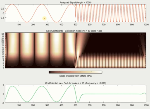
Coefficients may have redundant information since same feature may be captured by multiple scales.

CWT is suitable for detailed analysis and visualization of signals. NeuroAnalyzer uses CWT to calculate and plot scalogram.

Perform continuous wavelet decomposition (CWD):

cwd(e10, ch="all");

Wavelet Denoising

Denoising using continuous wavelet decomposition:

denoise_cwd(e10,
            ch="all",
            nf=50);

Tip: Denoising is performed by zeroing coefficients around the noise frequency and running inverse transform to reconstruct the signal.

Denoising using discrete wavelet decomposition:

denoise_dwd(e10,
            ch="all",
            smooth=:undersmooth,
            l=2);

l is the the number of decomposition levels.

smooth is the smoothing method used (:regular thresholds all given coefficients, whereas :undersmooth smoothing does not threshold the lowest frequency subspace node of the wavelet transform).

Tip: Default denoising function (dnt) is RelErrorShrink(SoftTH()). See WaveletsExt.jl for detailed description of available denoising functions.

Remove artifacts using continuous wavelet decomposition:

Before:

NeuroAnalyzer.plot(e10,
                   ch="Fp2",
                   ep=7)

plot_spectrogram(e10,
                 ch="Fp2",
                 ep=7,
                 flim=(0, 20))

Removing artifact at epoch 7:

e10_new = artrem_cwd(e10,
                     ch="Fp2",
                     ep=7,
                     tseg=(0.5, 2.5),
                     fseg=(0.5, 7.5))

Tip: Artifact position time segment must be provided within the epoch time, hence tseg=(0.5, 2.5) above.

Tip: Artifact removal is performed by zeroing coefficients around the artifact time and frequency and running inverse transform to reconstruct the signal.

After:

NeuroAnalyzer.plot(e10_new,
                   ch="Fp2",
                   ep=7)

plot_spectrogram(e10_new,
                 ch="Fp1",
                 ep=7,
                 flim=(0, 20))