
NeuroAnalyzer tutorials: Analyze: Stationarity
Initialize NeuroAnalyzer
using NeuroAnalyzer
using Plots
eeg = load("files/eeg.hdf")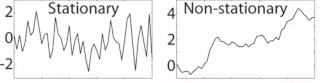
e10 = epoch(eeg, ep_len=10);Stationarity: statistical characteristics of the signal (mean, variance, frequency, autocovariance) stays similar over time
average power is constant over time
signal may maintain mean stationarity and does not have variance stationarity
Example: for a group of sampled signals (= ensemble), histograms of amplitudes are similar.
Ergodic process: when a single sampled signal is representative for the whole ensemble.
EEG is quasistationary - stationary only in short samples (10 seconds epoch is considered to be stationary).
EEG non-stationarity is due to changes in states of neuronal assemblies during brain functions (state of the brain evolves over time).
Non-stationarities in EEG signal are representative for underlying events.
Many signal processing methods require stationarity.
EEG may be segmented to achieve local stationarity:
- fixed segments
- adaptive methods
Stationarity can be used as a diagnostic tool for determining time windows for time-frequency analyses, because stationarity should be maintained for the length of time used for the analysis (this would correspond to the time window for the short-time Fourier transform or the temporal width of the Gaussian taper in Morlet wavelet convolution).
Mean stationarity: the time series can be divided into non-overlapping time windows, and then the mean of each window can be computed.
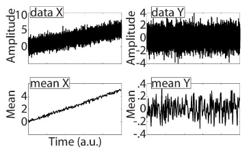
X: mean-non-stationarity
Y: mean-stationarity
Variance stationarity: normalize (using z score) the time series within each bin separately; this will produce non-continuous edges between bins, detrimental to subsequent analysis, unless analyses are performed separately in those bins.
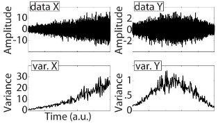
X: variance-non-stationarity
Y: variance-stationarity
Measurements of stationarity:
- skewness
- kurtosis
- neg-entropy
- Kullback-Keibler divergence = KL distance
If signal violates mean stationarity:
- detrend
- compute the derivative
- compute a time series of the time-varying mean and subtract that mean-time-series from the original time series
Stationarity can also be computed for higher-order moments such as skewness (asymmetries in variances) or kurtosis (the shape of the distribution ranging from flat to pointy), or any other statistical property of a time series.
Phase stationarity: unwrapped phase angle time series should increase monotonically and at a similar rate over time; frequency can be defined as the first temporal derivative of phase (instantaneous angular velocity), phase stationarity and frequency stationarity are overlapping concepts; phase stationarity = first temporal derivative (frequency) of the unwrapped phase angle time series should be positive and with similar values over time.
The signal should be filtered before interpreting phase stationarity.
Covariance stationarity is measured in non-overlapping time windows; for each time window a covariance matrix is compared to the covariance matrix from the previous time window; covariance stationarity will result in temporally successive covariances that are similar to each other; in contrast, covariance non-stationarity will result in successive covariances that are dissimilar.
Covariance matrices comparison (Euclidean distance metric): corresponding elements of the two covariance matrices are subtracted and squared, and all squared differences are summed (this can also be conceptualized as a sum of squared errors). The result are time series of distances between successive covariance matrices. This metric is compared against the time-varying means and variances of each individual time series.
Alternatively: compute the generalized eigenvalues between each two successive covariance matrices, and then take the distance as the ratio of the largest to the smallest eigenvalues
Statistical significance: mutual information method; quantifies the amount of information (entropy) that is shared between two time series: the time series of the stationarity variable (mean, variance, etc.) and time.
Works regardless of whether the relationship is linear or non-linear, positive or negative
Computes as entropy of variables X and Y minus their joint entropy (here, X and Y refer, respectively, to the non-stationarity variable and time)
\[ entropy = \sum(p \times \log(p)) \] \(p\): probability of observing a particular value in a particular bin (binning method: e.g. Freedman-Diaconis approach)
Mutual information result can be compared against a distribution of mutual information values that would be expected by chance, if there were no relationship between the stationarity variable and time - this distribution can be generated by randomly shuffling the time series and re-computing mutual information.
Other methods: tests for a “unit root”, which is related to the presence of significant autoregressive coefficients (that is, current values of the time series can be predicted from previous values), e.g. Augmented Dickey-Fuller test (ADF)
There are several types of stationarity tests available in NeuroAnalyzer.
To test mean stationarity:
s_m = stationarity(e10,
                   ch="eeg",
                   method=:mean,
                   window=256)
plot_signal(1:256,
            s_m[1, :, 1],
            xlabel="time-window points",
            title="channel 1, epoch 1")
To test variance stationarity:
s_v = stationarity(e10,
                   ch="eeg",
                   method=:var,
                   window=256)
plot_signal(1:256,
            s_v[1, :, 1],
            xlabel="time-window points",
            title="channel 1, epoch 1")
To test phase stationarity using Hilbert transformation:
s_p = stationarity(e10,
                   ch="eeg",
                   method=:hilbert,
                   window=256)
plot_signal(e10.epoch_time[1:end-1],
            s_p[1, :, 1],
            xlabel="Time [s]",
            title="channel 1, epoch 1")
To test covariance stationarity based on Euclidean distance between covariance matrix of adjacent time windows:
s_c = stationarity(e10,
                   ch="eeg",
                   method=:cov,
                   window=256)
plot_line(s_c[:, 15],
          xlabels=string.(1:length(s_c[:, 15])),
          label="epoch 15",
          ylabel="distance between covariance matrices",
          xlabel="time-window segment")
To test phase stationarity using Augmented Dickey–Fuller test:
s_adf = stationarity(e10,
                     ch="eeg",
                     method=:adf,
                     window=256)
s_adf[12, :, 1]
2-element Vector{Float64}:
-8.0
0.0001The output is ADF value and associated p value for channel 12, epoch 1. Significance of ADF value indicates stationarity.